The Season for Sharing Data: Working with the newly released Census 2010-2014 ACS 5 year data in R

On December 3, 2015 the U.S. Census Bureau released the 2010-2014 5 year ACS (American Community Survey) data. You can read all about it on the Census website. This fantastic five-year statistical database provides aggregate social and economic characteristics about American individuals and families down to the block group level. A number of online tools provide access to the ACS 2010-2014 data using graphical user interfaces (GUIs). These include the Census American FactFinder tool or via Social Explorer. The latter requires a subscription which UC Berkeley has and which is accessible to all folks with a CalNet login. Programmatic access to the data is possible via the Census API. In this blog post we will use the Census API to explore the ACS 2010-2014 data in the R statistical programming language.

It is not easy to work with Census data because of the size and the breadth of these data products. However, there are a number of packages that make it easier (but not easy!) to fetch, process and visualize Census data in R. These include the acs package by Ezra Glenn and the acs14lite package by Kyle Walker for downloading the ACS tabular data. The tigris package by Kyle Walker and Bob Rudis makes it relatively easy to download TIGER geographic boundary files, needed to map Census data, and link those boundaries to the ACS data.  Hadley Wickham's popular and powerful ggplot2 package can be used to make static maps and charts of the data. The ggmap package allows you to create maps of Google Maps data and other online reference maps that can be used as basemaps for our plots. The CartoDB-R package by Virgilio Gómez-Rubio, which extends the work of Andrew Hill and Kyle Walker, makes it super easy to create online interactive maps of these data using the CartoDB.com APIs. The sp, rgdal and rgeos libraries are the workhorses of spatial data operations in R and are libraries upon which other packages may depend.

This tutorial has been tested with R version 3.2.2 (2015-08-14) on MacOSX 10.9.5. You may need to update your R to follow along. Ok, let's get started.

First, open RStudio or similar R development enviroment. Install the packages we will use if they are not already on your system. Some of these need to be installed with devtools which facilitaties installing packages that are not  in a CRAN repository. You only do the package install once.

install.packages(c('dplyr','ggplot2','ggmap','sp','rgdal','rgeos','maptools','devtools'))
devtools::install_github('walkerke/acs14lite')
devtools::install_github('walkerke/tigris')
devtools::install_github('becarioprecario/cartodb-r/CartoDB', dep=TRUE)

Now load the libraries. A library is the code part of an R package which may also include documentation, data, and tests, etc.

library(sp) # for working with spatial data objects
library(rgdal) # for importing and exporting spatial data in various formats
library(acs14lite) # used to fetch ACS data
library(tigris) # used to fetch TIGER data (shapefiles)
library(dplyr) # used to reformat the ACS data
library(maptools) # used by ggplot and base maps
library(ggplot2) # used to make maps of the ACS data
library(ggmap) # for adding Google Maps data to our maps
library(CartoDB) # to create interactive maps in CartoDB.com

Set your working directory on your local computer

setwd('~/Documents/census') #mac style
#setwd("c:/docs/mydir") #windows os stye

my_census_api_key <- "your api key"
set_api_key(my_census_api_key)

sf_poverty <- acs14(geography = 'tract', state = 'CA', county = 'San Francisco', 
                 variable = c('B17021_001E', 'B17021_001M', 'B17021_002E', 'B17021_002M'))

head(sf_poverty) # view retrieved data

sf_poverty14 <- mutate(sf_poverty,
                    geoid = paste0(state, county, tract),
                    pctpov = round(100 * (B17021_002E / B17021_001E), 1),
                    moepov = round(100 * (moe_prop(B17021_002E, B17021_001E, B17021_002M, B17021_001M)),1))
sf_poverty14 <- select(sf_poverty14, geoid, pctpov, moepov)

head(sf_poverty14) # take a look at the retieved and reformatted ACS data

sf_tracts <- tracts('CA', 'San Francisco', cb=TRUE)

sf_tracts2 <- geo_join(sf_tracts, sf_poverty14, "GEOID", "geoid")
sf_tracts2 <- sf_tracts2[!is.na(sf_tracts2$pctpov),]
# look at the data
class(sf_tracts2)
str(sf_tracts2)
str(sf_tracts2@data)

# First use fortify() to make the spatial data object a data frame that ggplot can map.
ggplotData <- fortify(sf_tracts2, data=sf_tracts2@data, region="geoid")
head(ggplotData) # look at the data frame created with the fortify function

# Join the ACS data to the fortified data frame
ggplotData <- merge(ggplotData, sf_tracts2@data, by.x="id", by.y="geoid")
head(ggplotData) # look at the data

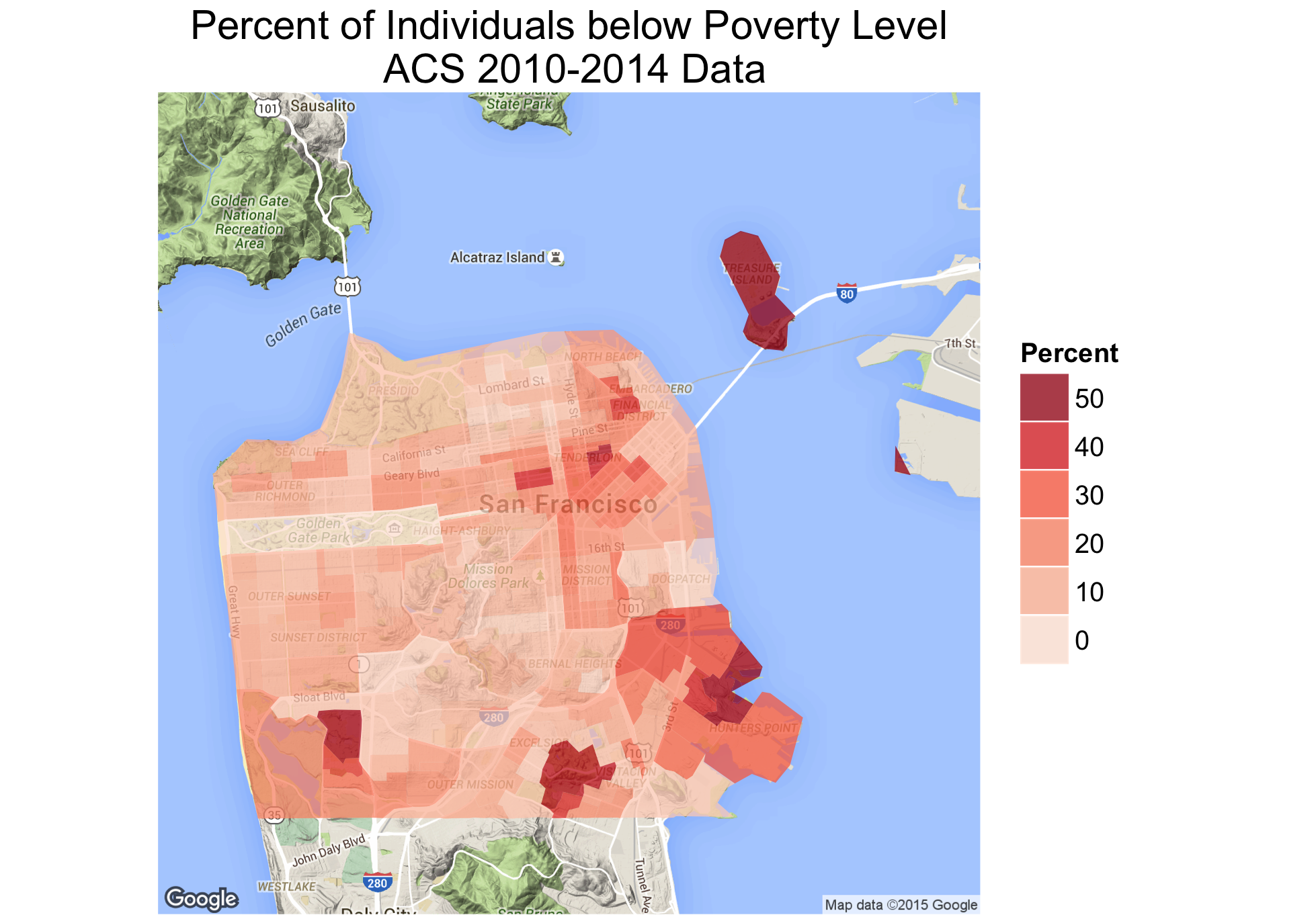
# Plot the data to emphasize the areas of highest poverty
# First use the ggmap get_map function to fetch a Google Map image to use as our basemap
sf_basemap <-get_map('San Francisco', zoom=12) 
ggmap(sf_basemap) +
  geom_polygon(data = ggplotData, aes(x = long, y = lat, group = group, fill = pctpov), alpha=0.75) +
  scale_fill_distiller(palette = "Reds") +
  guides(fill = guide_legend(reverse = TRUE)) +
  ggtitle("Percent of Individuals below Poverty Level\n ACS 2010-2014 Data") +
  theme_nothing(legend=TRUE) +
  coord_map()

library(CartoDB)
cdb_username <- 'your_username'
cdb_apikey <- 'your_apikey'
cartodb(cdb_username, cdb_apikey)
r2cartodb(sf_tracts2, 'sf_poverty_by_tract')